# Impoort the libraries
import math
import pandas_datareader as web
import numpy as np
import pandas as pd
from sklearn.preprocessing import MinMaxScaler
from keras.models import Sequential
from keras.layers import Dense,LSTM
import matplotlib.pyplot as plt
plt.style.use('fivethirtyeight')
C:\Python\Python38\lib\site-packages\pandas_datareader\compat\__init__.py:7: FutureWarning: pandas.util.testing is deprecated. Use the functions in the public API at pandas.testing instead.
  from pandas.util.testing import assert_frame_equal
Using TensorFlow backend.
#get the stoke quote
df = web.DataReader('RBS.L',data_source='yahoo',start='2010-01-01',end='2020-04-29')
#show the data
df
| High | Low | Open | Close | Volume | Adj Close | |
|---|---|---|---|---|---|---|
| Date | ||||||
| 2010-01-04 | 321.000000 | 295.000000 | 299.000000 | 321.000000 | 11667982.0 | 299.654846 |
| 2010-01-05 | 355.000000 | 318.000000 | 320.000000 | 354.000000 | 18885923.0 | 330.460480 |
| 2010-01-06 | 384.899994 | 355.000000 | 357.200012 | 366.799988 | 19304534.0 | 342.409332 |
| 2010-01-07 | 371.000000 | 354.500000 | 366.799988 | 358.700012 | 14208016.0 | 334.847961 |
| 2010-01-08 | 366.500000 | 346.600006 | 365.500000 | 351.200012 | 10188018.0 | 327.846680 |
| ... | ... | ... | ... | ... | ... | ... |
| 2020-04-23 | 1.070000 | 1.035500 | 1.049500 | 1.064500 | 19678442.0 | 1.064500 |
| 2020-04-24 | 1.069000 | 1.038500 | 1.063500 | 1.046000 | 19949004.0 | 1.046000 |
| 2020-04-27 | 1.086500 | 1.043000 | 1.082500 | 1.075000 | 22654143.0 | 1.075000 |
| 2020-04-28 | 1.172000 | 1.055500 | 1.071000 | 1.150500 | 38581905.0 | 1.150500 |
| 2020-04-29 | 120.485901 | 114.099998 | 116.050003 | 120.449997 | 33760944.0 | 120.449997 |
2603 rows × 6 columns
df.shape
(2603, 6)
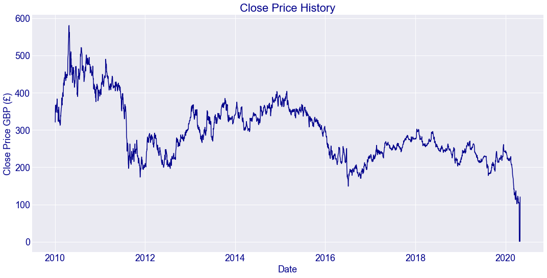
#visualise the closing price graph
plt.style.use('seaborn-darkgrid')
plt.figure(figsize=(16,8))
plt.title('Close Price History',color='darkBlue',fontsize=22)
plt.plot(df['Close'],linewidth=1.5,color='darkBlue')
plt.xlabel('Date',fontsize=18,color='darkBlue')
plt.ylabel('Close Price GBP (£)',fontsize=18,color='darkBlue')
plt.xticks(color='darkBlue',fontsize=18)
plt.yticks(color='darkBlue',fontsize=18)
plt.show()
#Create a new dataframe with only the Close column
data = df.filter(['Close'])
#Converty the dataframe to a numpy array
dataset = data.values
#get the number of rows to train the model on
training_data_len = math.ceil(len(dataset)*.8)

training_data_len
2083
#Scale the data
scaler = MinMaxScaler(feature_range=(0,1))
scaled_data = scaler.fit_transform(dataset)
scaled_data
array([[5.52164624e-01],
       [6.09114787e-01],
       [6.31204527e-01],
       ...,
       [5.00471890e-05],
       [1.80342280e-04],
       [2.06062944e-01]])
#Create the training data set
#Create the scaled training data set
train_data = scaled_data[0:training_data_len , :]
#Split the data into x_train and y_train data sets
x_train = []
y_train = []

for i in range(60, len(train_data)):
  x_train.append(train_data[i-60:i, 0])
  y_train.append(train_data[i, 0])
  if i<=60:
    print(x_train)
    print(y_train)
    print()
[array([0.55216462, 0.60911479, 0.63120453, 0.61722589, 0.60428267,
       0.60186656, 0.59841504, 0.61256631, 0.61946936, 0.63223999,
       0.64086881, 0.6598522 , 0.65398461, 0.6077342 , 0.59668928,
       0.60842449, 0.59876021, 0.59099428, 0.56027573, 0.55561615,
       0.59979568, 0.62205801, 0.60876961, 0.57339148, 0.55509844,
       0.55302751, 0.5480228 , 0.56079344, 0.56079344, 0.53749564,
       0.54353581, 0.57218348, 0.58322835, 0.58046712, 0.59410063,
       0.61567266, 0.61946936, 0.62171283, 0.66451178, 0.64828962,
       0.63137711, 0.64949762, 0.65260402, 0.67745499, 0.68832728,
       0.67935334, 0.67089706, 0.69540291, 0.69799156, 0.73285198,
       0.73561316, 0.74510485, 0.74976443, 0.72301511, 0.75753036,
       0.75373367, 0.75856583, 0.76598659, 0.78514257, 0.78496998])]
[0.7709912914434884]
#Convert the x_train and y_train to numpy arrays
x_train, y_train = np.array(x_train),np.array(y_train)
#reshape the data
x_train = np.reshape(x_train,(x_train.shape[0],x_train.shape[1],1))
x_train.shape
(2023, 60, 1)
#Build the LSTM model
model = Sequential()
model.add(LSTM(50, return_sequences=True, input_shape=(x_train.shape[1],1)))
model.add(LSTM(50,return_sequences=False))
model.add(Dense(25))
model.add(Dense(1))
#Compile the model
model.compile(optimizer='adam', loss = 'mean_squared_error')
#Train the model
model.fit(x_train,y_train,batch_size=1,epochs=1)
Epoch 1/1
2023/2023 [==============================] - 92s 46ms/step - loss: 0.0015


<keras.callbacks.callbacks.History at 0x2b2d73e6e80>
#Create the testing data set
#Create a new array containing scaled values from index 2020 to 2080
test_data = scaled_data[training_data_len-60: , :]
#Create the data set x_test and y_test
x_test = []
y_test = dataset[training_data_len:, :]
for i in range(60, len(test_data)):
  x_test.append(test_data[i-60:i, 0])
#Convert the data to a numpy array
x_test = np.array(x_test)
#Reshape the data
x_test = np.reshape(x_test,(x_test.shape[0],x_test.shape[1], 1))
#Get the models predicted price values
predictions = model.predict(x_test)
predictions = scaler.inverse_transform(predictions)
#Get the root mean squared error(RMSE)
rmse = np.sqrt(np.mean(predictions - y_test)**2)
rmse
4.338851857643861
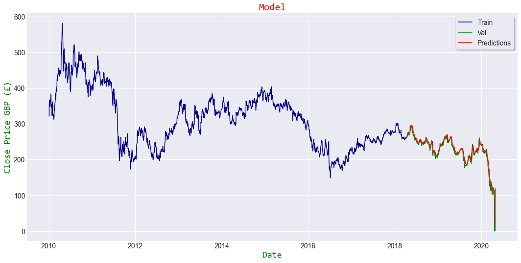
#Plot the data
train = data[:training_data_len]
valid = data[training_data_len:]
valid['Predictions'] = predictions

#Visualise the data
plt.style.use('seaborn-darkgrid')
plt.figure(figsize=(16,8))
plt.title('Model',color='red',fontname='Consolas')
plt.xlabel('Date',fontsize=18,color='green',fontname='Consolas')
plt.ylabel('Close Price GBP (£)',fontsize=18,color='green',fontname='Consolas')

plt.plot(train['Close'],linewidth=1.5,color='darkBlue')
#plt.plot(valid[['Close','Predictions']],linewidth=1.5)
plt.plot(valid.Close,linewidth=1.5,color='green') #real price
plt.plot(valid.Predictions,linewidth=1.5,color='red') #estimated price

plt.legend(['Train','Val','Predictions'], loc='upper right',frameon=True,fancybox=True,shadow=True,framealpha=1)
plt.show()
<ipython-input-18-4f6b43f84d62>:4: SettingWithCopyWarning:
A value is trying to be set on a copy of a slice from a DataFrame.
Try using .loc[row_indexer,col_indexer] = value instead

See the caveats in the documentation: https://pandas.pydata.org/pandas-docs/stable/user_guide/indexing.html#returning-a-view-versus-a-copy
  valid['Predictions'] = predictions
#show the valid and predicted prices
valid
| Close | Predictions | |
|---|---|---|
| Date | ||
| 2018-04-11 | 263.200012 | 264.371277 |
| 2018-04-12 | 264.700012 | 265.043915 |
| 2018-04-13 | 264.799988 | 265.859009 |
| 2018-04-16 | 262.899994 | 266.557800 |
| 2018-04-17 | 268.399994 | 266.636963 |
| ... | ... | ... |
| 2020-04-23 | 1.064500 | 92.099251 |
| 2020-04-24 | 1.046000 | 70.637138 |
| 2020-04-27 | 1.075000 | 51.948002 |
| 2020-04-28 | 1.150500 | 37.720310 |
| 2020-04-29 | 120.449997 | 27.833059 |
520 rows × 2 columns
#Get the Quote
rbs_quote = web.DataReader('RBS.L',data_source='yahoo',start='2010-01-01',end='2020-04-29')
#Create a new dataframe
new_df = rbs_quote.filter(['Close'])
#Get the last 60 days closing price and convert the dataframe to an array
last_60_days = new_df[-60:].values
#Scale the data to be values between 0 and 1
last_60_days_scaled = scaler.transform(last_60_days)
#Create an empty list
X_test = []
#Append the last 60 days to the list
X_test.append(last_60_days_scaled)
#convert the X_test dataset to a numpy array
X_test = np.array(X_test)
#Reshape the data
X_test = np.reshape(X_test,(X_test.shape[0],X_test.shape[1], 1))
#Get the predicted scaled price
pred_price = model.predict(X_test)
#Undo the scaling
pred_price = scaler.inverse_transform(pred_price)
print(pred_price)
[[39.654922]]
#Get the quote
rbs_quote2 = web.DataReader('RBS.L',data_source='yahoo',start='2020-04-29',end='2020-04-29')
print(rbs_quote2['Close'])
Date
2020-04-29    120.449997
Name: Close, dtype: float64